ket1 <- qstate(nbits=2, coefs=c(6,3,4,7))
ket1
( 0.5720775535473555 ) * |00>
+ ( 0.2860387767736777 ) * |01>
+ ( 0.381385035698237 ) * |10>
+ ( 0.6674238124719146 ) * |11> sum(Mod(ket1@coefs)^2)[1] 1I think I will continue in some linear algebra, but reconnecting to quantum definitions. So, let’s start this post with some postulates.
Postulate 1: Associated with any isolated physical system is a complex vector space with inner product1 known as the state space of the system. The system is completely described by its state vector, which is a unit vector in the system’s state space.
Postulate 2: The evolution of a closed quantum system is described by a unitary transformation. that is, the state \(|\psi>\) of the system at time t1 is related to the state \(|\psi'>\) of the system at time t2 by a unitary operator U which depends only on the times t1 and t2.
\[|\psi'> = U |\psi>.\]
Postulate 2 requires that the system described is closed, and does not react with any other system. In reality that is rarely the case. The above postulates are described in greater detail on pages 80, 81 of (Nielsen and Chuang 2010).
In linear algebra, eigenvalues are described in the vector equation
\[ Ax = \lambda x\]
where A is a given square matrix, \(\lambda\) is an unknown scalar, and x an unknown vector. The task is to determine \(\lambda\)’s and x’s that satisfy the above formula, where \(x \ne 0\). The \(\lambda\) values that satisfy the above formula are called eigenvalues of A, and the x solutions are called eigenvectors of A.
So, if we had a matrix and vector(s) as below and wished to multiply to determine a vector in the same direction as the original vector and satisfy the above equation, as such
\[\begin{bmatrix} 6& 3 \\ 4& 7 \end{bmatrix} \begin{bmatrix} 5 \\ 1 \end{bmatrix} = \begin{bmatrix} 33 \\ 27 \end{bmatrix}, \qquad \begin{bmatrix} 6& 3 \\ 4& 7 \end{bmatrix} \begin{bmatrix} 3 \\ 4 \end{bmatrix} = \begin{bmatrix} 30 \\ 40 \end{bmatrix} \]
We can see the second vector does, where \(\lambda = 10\) and x = [3 4]T2 and A, the 2x2 matrix, is proportional to x. As can be seen, the first vector is not. In R, we multiply as so: \(\quad A \quad \%*\% \quad \lambda\).
Looking at the second example, we see the linear equation as
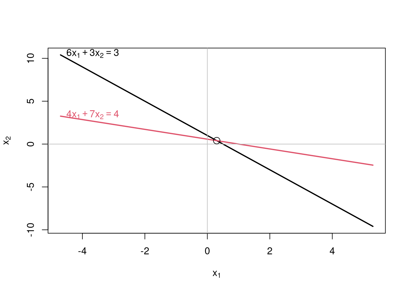
\[\begin{equation}\begin{split}6x_{1} + 3x_{2} = 3 \\ 4x_{1} + 7x_{2} = 4\end{split}\end{equation}\]
where \(x_{1}\) = 0.3 and \(x_{2}\) = 0.4, found by reduced row echelon format (RREF) of the augmented matrix3. See also The Matrix for more. Also, similar to Part 3, we plot the linear equations. The circle indicates the solution.
And, the eigenvalues of a unitary matrix (complex generalization of an orthogonal matrix) have eigenvalues that are complex numbers with modulus 1. So, to check that, let’s create a two-qubit state using the above matrix as such
ket1 <- qstate(nbits=2, coefs=c(6,3,4,7))
ket1 ( 0.5720775535473555 ) * |00>
+ ( 0.2860387767736777 ) * |01>
+ ( 0.381385035698237 ) * |10>
+ ( 0.6674238124719146 ) * |11> sum(Mod(ket1@coefs)^2)[1] 1and the result is 1. If we then introduce a BELL state to this ket1, we see the result below. Is this a state of superdense coding?
z <- CNOT(c(1,2)) * (H(1) * ket1)
show(z)
( 0.606779876216918 ) * |00>
+ ( -0.2022599587389726 ) * |01>
+ ( 0.7416198487095663 ) * |10>
+ ( 0.2022599587389727 ) * |11> plot(z)
And does it meet the validity test where the coefficients squared equal 1?
sum(Mod(z@coefs)^2)[1] 1We could carry this on with even more qubits, but it serves no purpose here. So now it’s back to the books for more.
Have a great day, and may the Lord Bless you. If you haven’t accepted Jesus as your Lord and Savior, there’s no time like the present. Don’t wait until it’s too late!