The Matrix
As this is a ‘snow day,’ I decided to explore some matrix operations, otherwise known as linear algebra. In this case, I am using an electronic circuit to determine how mesh currents may flow in the various branches. I am not very familiar with matrix operations, but I will use them in a casual way to determine the various values of current flow in a classic circuit that folks many times use to demonstrate how resistors interact in a series/parallel circuit. I will use only the major branch currents and not the sub-branches as it makes for an easier job to illustrate my point. And, this is to help my understanding as well!
Firstly, Kirchhoff’s Current Law states that at any point of a circuit, the sum of inflowing currents equal the sum of the outflowing currents. The Voltage Law states that in a closed loop, the sum of all voltage drops equals the applied voltage.
A really nice thing about matrix operations is it makes for much easier going for things like least squares calculations, such as land surveying data reduction. Although I have not managed to use least squares for surveying yet, I have hopes to do so someday. But that is not what I am doing in this post.
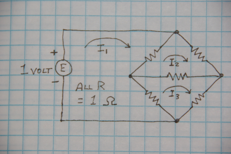
As shown in the above circuit, a voltage is connected in what is very similar to a wheatstone bridge circuit. The arrows I used are for circuit current flow to choose a direction for determining the formulas, and may change after final reduction. I was first presented with this particular circuit as an exercise back in my 20s to figure the total resistance. At that time I had no clue! So, I actually built the circuit to measure it! In any case, this is the circuit I will use for this effort. Looking at the various branch currents, one is able to determine some formulas for each branch, presented below. As noted in the image, all resistances are 1\(\Omega\) and the applied voltage is 1 Volt.
\[I_1: 2x -1y -1z = -1\] \[I_2: -1x +3y -1z = 0\] \[I_3: -1x -1y +3z = 0\] Note: One circuit not shown would be around the outside, but in this case, it would be identical with the first.
We place the resistance values in a ‘square matrix’ or ‘coefficient matrix’, and combine the voltage vector to create the following structure.
\[\begin{bmatrix} 2& -1& -1 \\ -1& 3& -1 \\ -1& -1&3 \end{bmatrix} + \begin{bmatrix} -1\\0\\0 \end{bmatrix} = \begin{bmatrix} \underline{+2}& -1& -1& |& -1 \\ -1& \underline{+3}& -1& |& 0 \\ -1& -1& \underline{+3}& |& 0 \end{bmatrix}\]
The above matrix is known as an augmented matrix and contains all the numbers necessary to determine the results. The first three columns contain the resistance values and the last column (a vector) contains the voltage at the end of each current loop. As you travel around each loop, you tabulate the values, either added or subtracted from the total for that loop. Each formula is created to identify each unknown (x,y,z, etc). Taking the first loop as an example, the first underlined position is the ‘x’ value, which totals the resistance (2\(\Omega\)); and, since the other resistances are part of other loops, they are depicted as negative values. The last (vector) column is the voltage, and is negative, as it ends at the minus side of the power source. If the voltage were reversed, it would be positive.
For the other formulas, the second underlined position (row 2) is the ‘y’ value; for the final formula the third (row 3) is ‘z.’
Several operations can be performed here to make things easier. The first I will do is called ‘Gauss Elimination’ method. This is used to transform the matrix into an upper triangular format where all entries below the pivot line are zero, and the remaining ‘real’ values are above. The below example shows the result of the first step where I will multiply the first row by 0.5 and add to the second row. This leaves a zero in the first position of the second row. Note when I mention performing a particular operation on a row value, it applies to all the row values of that row and any affected rows.
\[\begin{bmatrix} +2& -1& -1& -1 \\ 0& 2.5& -1.5& -0.5 \\ -1& -1&+3& 0 \end{bmatrix}\]
Next, we will change the middle position of the third row to zero by multiplying the second row value (2.5) by 0.4 and adding to the third row. This will place the matrix in a ‘row echelon form’ where zeros fill the lower left.
\[\begin{bmatrix} +2& -1& -1& -1 \\ 0& 2.5& -1.5& -0.5 \\ 0& 0& 1.6& -0.8 \end{bmatrix}\]
At this point you could continue with back substitution to determine x,y,z, but another more efficient way is to start by converting the rows to ones as the calculations then become easier. For example, the first position of the original matrix (2) can be converted to 1 by multiplying by 0.5. This makes the original matrix as shown.
\[\begin{bmatrix} \underline{+2}& -1& -1& -1 \\ -1& \underline{+3}& -1& 0 \\ -1& -1& \underline{+3}& 0 \end{bmatrix} becomes \begin{bmatrix} 1& -0.5& -0.5& -0.5 \\ -1& 3& -1& 0 \\ -1& -1& 3& 0 \end{bmatrix}\]
Then, simply adding row one to rows two and three converts to zero the first column of each formula. Then multiply the second row, second column value (2.5) by 0.4 to convert to one.
\[\begin{bmatrix} 1& -0.5& -0.5& -0.5 \\ 0& 2.5& -1.5& -0.5 \\ 0& -1.5& 2.5& -0.5 \end{bmatrix} becomes \begin{bmatrix} 1& -0.5& -0.5& -0.5 \\ 0& 1& -0.6& -0.2 \\ 0& -1.5& 2.5& -0.5 \end{bmatrix}\]
Next, place a zero in the third row, second column by multiplying the second row, second column value by 1.5 and adding to the third column.
\[\begin{bmatrix} 1& -0.5& -0.5& -0.5 \\ 0& 1& -0.6& -0.2 \\ 0& -1.5& 2.5& -0.5 \end{bmatrix} to\:get \begin{bmatrix} 1& -0.5& -0.5& -0.5 \\ 0& 1& -0.6& -0.2 \\ 0& 0& 1.6& -0.8 \end{bmatrix}\]
Then, for the last row reduction, multiply 1.6 by 0.625 for the last ‘1’ which shows ‘z’ as -0.5.
\[\begin{bmatrix} 1& -0.5& -0.5& -0.5 \\ 0& 1& -0.6& -0.2 \\ 0& 0& 1.6& -0.8 \end{bmatrix} is \begin{bmatrix} 1& -0.5& -0.5& -0.5 \\ 0& 1& -0.6& -0.2 \\ 0& 0& 1& -0.5 \end{bmatrix}\]
And once again we have the ‘row echelon form’ of the equation. Alternativly, to determine the value of ‘z,’ reduce row three: \(z = \frac{-0.8}{1.6} = -0.5\), which shows there are more than one way to ‘skin a cat’ as an old saying depicts.
Contiuing with back substitution, we can then take the second formula like so to find the ‘y’ value: \(1 + (-0.6z) / -0.2 = -0.5\)
This leaves only the ‘x’ value which is determined the same way: \(x = -0.5 / (-0.5y + -0.5z) = -1\). The final vectors for unknowns x,y,z are:
\[\begin{bmatrix} -1 \\ -0.5 \\ -0.5 \end{bmatrix}\]
Since the unknown values are determined to be negative, this means the actual current flow is opposite the direction we depicted with the arrows on the diagram. And, oh by the way, the total resistance of the circuit is 1\(\Omega\).
Now, having gone through this entire process, I have to point out that many graphics calculators have functions to perform reduced row echelon form (RREF) calculations by pressing a few keys. For example, I prefer Casio Prizm calculators, which do that by a simple ‘RREF Mat x.’ That, however leaves one in the dark about HOW the process is actually done! And what’s the fun in that?
It is a bit difficult to keep track of the various stages of the reduction, so I hope I haven’t made mistakes. If so, well, it is what it is…
We thank the Lord Jesus for all we have and continue to ask for guidance and direction in our lives, especially how we interact with others. And now the ‘show day’ seems to be continuing. We thought it was over as the sun was out and melted all the snow, but now it has started again! So, if you must be out, drive safely! Until next time…