Quantum Investigations Part 1

Author

Sam Hutchins

Published

September 3, 2023

Wow, how time flies when you’re having fun! We sit back and technology advances.. So now it’s time to leap into the fast-developing concept of Quantum Mechanics. Where do we start? Well, it seems like the beginning might be a starting point. WARNING: This may get into Linear Algebra and matrices as we attempt to understand all this. Also expect mistakes, errors and misconceptions as I try to jump into this. It’s an Adventure !

Beginnings

I suppose we should look at, “just what is a qubit?” A qubit (quantum bit) is a quantum system whose classical state is 0, 1. It’s just a bit, but it can be in a quantum state 3 (superposition). NOTE: There are reams of information about this subject on the Internet, so this is mostly done for my own understanding, not to present new information.

A valid quantum state vector must be such that the sum of the absolute values squared of the entries must be equal to 1. To manipulate the qubits (such as kets and bras), I will use the R package, qsimulatR, which is a quantum simulator for R. BTW, there is a nice four-part series posted on R-Bloggers that goes a long way explaining the operation and usage of the qsimulatR package. The original series shows all four parts.

Now, using qsimulatR, I will define a qubit |0〉.

ket0 <- qstate(nbits=1)
ket0

   ( 1 )    * |0>

There are a couple of ways to define a qubit |1〉. The easiest way is using a Pauli X gate (bit flip).

ket1 <- X(1) * ket0
ket1

   ( 1 )    * |1>

The other way is define the coefficients, obviously more cumbersome.

ket1 <- qstate(nbits=1, coefs=c(0,1))

To compute the sum of the absolute values squared of a quantum state vector, we can use the Mod() function.

sum(Mod(ket0@coefs)^2)

[1] 1

which shows a valid 1. I’ve been a bit remiss in not showing where the coefficients (and other elements) are coming from. To display the internal structure of an R object, such as a qubit, we can use the str command from the utils package.

str(ket0)

Formal class 'qstate' [package "qsimulatR"] with 5 slots
  ..@ nbits  : int 1
  ..@ coefs  : cplx [1:2] 1+0i 0+0i
  ..@ basis  : chr [1:2] "|0>" "|1>"
  ..@ noise  :List of 4
  .. ..$ p    : num 0
  .. ..$ bits : int 1
  .. ..$ error: chr "any"
  .. ..$ args : list()
  ..@ circuit:List of 2
  .. ..$ ncbits  : num 0
  .. ..$ gatelist: list()

So that’s where the coefficients are that add to 1 as noted above.

Superposition

Superposition is a complete entanglement of a qubit |0〉 and |1〉 states, represented by | $ψ$ 〉 (psi), the range of potential states, all at once, but weighted to acknowledge that some states are more likely to occur than others.

$| ψ > = 1 + 2 i 3 | 0 > 23 | 1 >$

This entanglement, following the above formula, is accomplished by defining the coefficients for each bit, |0> and |1>, as shown here.

psi <- qstate(nbits=1, coefs=c((1+2i)/3, -2/3))
psi

   ( 0.333333333333333+0.666666666666667i ) * |0> 
 + ( -0.666666666666667+0i )    * |1>

And to verify | $ψ$ 〉 is a valid quantum state vector we sum the absolute values squared to get 1.

sum(Mod(psi@coefs)^2)

[1] 1

Also, any valid quantum gate must be reversible.

Quantum gates have to be reversible because quantum mechanics is reversible (and even more specifically it is unitary). It’s just an observed fact about the universe. (Even measurement can be modeled as a reversible unitary operation, inconvenient though that may be.)

Another aspect of entanglement is that two entangled particles, regardless of distance between, are related to each other when measured. So if a particle is measured as ‘spin up’, the other, when measured at the exact same time, will be ‘spin down.’ Referring to distance, that could be many light years apart. All this is very non-intuitive!

Measurements

The act of measuring a quantum circuit collapses the quantum state to a classical state and only gives probabilities of an answer, not a 0 or 1 answer as in classical computer gates. What this means is an attempt to actually measure a probability state, destroys that state. So, just for the fun of it, here is Schrodinger’s equation. To find the motion of a particle with total energy $E$ , moving in one dimension, $x$ , in a region in which there is a potential, $V$ , where probability amplitudes are represented by the above-mentioned Greek letter psi ( $ψ$ ). Particle mass is $m$ , $ℏ$ is Planck’s constant¹ $h$ divided by $2 π$ .

$E ψ = - ℏ 2 2 m d 2 ψ d x 2 + V ψ$

That reminds me of the paradox of Schrodinger’s cat. But that’s another story, although it does illustrate the difficulty of observing something that can’t be observed without changing the possible outcome (waveform collapse).

Gates

In constructing a quantum circuit, many gates are available, which allow circuits to replicate similar classical circuits such as $a n d$ , $n a n d$ , $o r$ , $x o r$ and $n o t$ gates. These gates are, in no particular order, the Hadamard $H$ gate, the Pauli $X$ , $Z$ , $Y$ gates, the $S$ and $T$ gates. The motion and action of these gates can be represented on a Bloch sphere, depicted below.

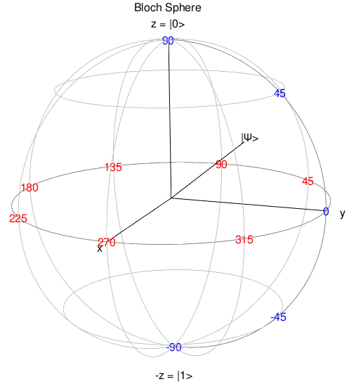
So, what function does each gate perform? The list below briefly describes each gate’s action.

H gate creates a uniform superposition of the quantum state.
Pauli X gate performs a bit flip (classical NOT operation).
Pauli Z gate performs a phase flip on |1> state relative to the |0> state, generating a half-turn about the z-axis.
Pauli Y gate performs a bit and phase flip (combination of X and Z gates), generating a half-turn about the y-axis.
S gate shifts the phase of |1> state relative to |0> state, adding $90 o$ rotation of the phase about the z-axis.
T gate performs 1/4th of the Z gate and 1/2 of the S gate, performing an eighth-turn anti-clockwise about the z-axis.
CNOT gate (Controlled-NOT) is used in Grover’s Algorithm, not discussed in this post.

All these actions can be demonstrated on the Bloch sphere.

I think perhaps there may be more segments to this post. Check back. We praise God for all things, because He surpasses all of man’s understanding. Be safe!

Footnotes

Planck’s constant is the fundamental constant of quantum mechanics and is extremely small: $6.6260693 (11) x 10 - 34$ ↩︎
I constructed the Bloch sphere using the rgl and sphereplot packages.↩︎