Helmholtz Coil
I admit I love to include formulae in many posts because it is so much fun to figure how using Allaire et al. (2023) and Latex math. Do I sometimes overdo it? Most likely! Why do I do it this way? Simple, for my edification and so I can refer back to it at some later date possibly.
This post is about the Helmholtz coil. There is lots of wonderful information on Wikipedia about the procedures involved and how to determine the field strengths at various locations in and around the coils.
The one I acquired is simple, just two coils on a rail to allow the spacing to be adjusted.
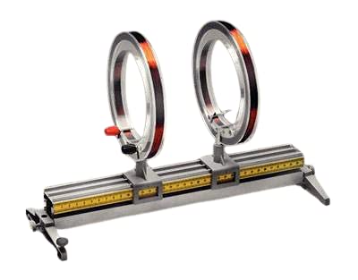
One thing I haven’t tried is feed a frequency instead of just DC to the coils, or feed in opposite directions, known as an anti-Helmholtz coil, which as I understand, can be used to trap particles, atoms, or the like.
So, to find the value of the magnetic field at the center, as in this post, the below formula is used,
\[B = \left(\frac{4}{5}\right)^{3/2} \frac{\mu_{o} n I}{R}\]
where \(\mu_{o}\) is the permeability of free space (or magnetic constant) of \(4\pi\times10^{-7}\) or \(12.566370614\times10^{-7}\), \(n\) is number of turns in each coil, \(I\) is current, and \(R\) is the radius of the coil, where we want the coil spacing the same as \(R\). If we use 0.5 A, we get a magnetic field strength of 64 uA/meter (H). For these coils, maximum current is 1A, giving 128 uA/m.
For a DC static field, the strength of the magnetic field is proportional to the current (I). However, if I wish to generate a variable frequency field, I have to consider the inductance of the coils, as the impedance is proportional to the frequency,
\[X_{L} = 2\pi f L, \quad and \quad |Z| = \sqrt{R^{2} + X_{L}^{2}}\]
where \(f\) is frequency, L is inductance, R is coil resistance, and |Z| is the absolute value of impedance. To duplicate the direct current (DC) field strength, a waveform/RF amplifier is required1 to feed the coils. The formula to calculate the required current is,
\[I = \left(\frac{5}{4}\right)^{3/2} \left(\frac{BR}{\mu_{o} n}\right)\]
where R is coil radius, n is number of turns in each coil. For 0.5 A DC, this gives 0.5 A waveform current required. For the amplifier voltage,
\[V = I \sqrt{[\omega(L_{1} + L_{2})]^{2} + (R_{1} + R_{2})^{2}}\]
where the angular frequency, \(\omega = 2 \pi f\), and the L’s and R’s are the coil’s inductances and resistances, respectively. This seems to give a rather large voltage value (>7.8 kV @ 0.5 A), so I may have erred.
Firstly, I want to experiment with a 6” plasma globe to see the effect for various positions and distances within the magnetic field. That may or may not be interesting.
Let’s see what we can determine for the Helmholtz coil. For a multilayer coil, from Richard C. Dorf (1997), the Wheeler2 formula for multilayer coils, formula 1.47, p.25, is,
\[L = \frac{0.8 B^{2} N^{2}}{6B + 9A + 10C} \quad \mu H\]
where \(B\) is winding radius, \(N\) is number of turns, \(A\) is width of winding, and \(C\) is height of winding. These are the dimensions of one coil,
- Radius (B) = 2.805”
- Width (A) = 0.525”
- Height (C) = 0.33”
- Turns (N) = 400
- Resistance (R) = 19.3 \(\Omega\)
When we plug these values into the above formula, we get an inductance of 43.598 mH, with an error range of < 5%, which is 41.42 mH3. At DC, the inductive reactance, \(X_{L} = 2 \pi f L =0.26 \Omega\), giving an impedance,
\[Z = \sqrt{R^{2} + X_{L}^{2}} = 19.3 \Omega \equiv R\]
Let’s see if we can determine the self-resonant frequency (SRF) for the coil. The inductance is in series with the coil resistance and in parallel with the parasitic capacitance. As we know that at the resonant frequency, \(X_{L} = X_{C}\), and \(f = \frac{1}{2 \pi \sqrt{LC}}\), we can find the parasitic capacitance.
\[\omega = \sqrt{\frac{1}{LC} - \frac{R^{2}}{L^{2}}} \quad or \quad \frac{1}{\sqrt{LC}} \sqrt{1 - \frac{R^{2} C}{L^{2}}}\]
where \(\omega\) is self-resonant frequency. The first formula gives 62.465 kHz, the second 62.425 kHz. To check these, we will use the nanoVNA.
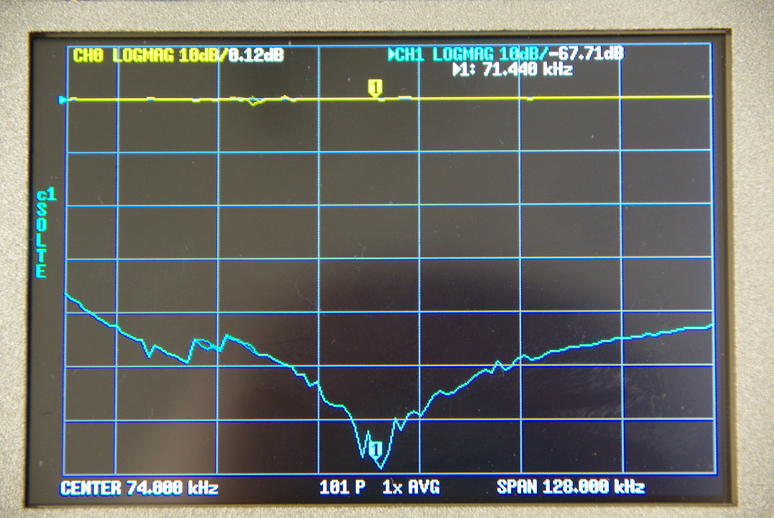
This image seems to indicate the self-resonant point approximately, but the leads I had to use were rather long, so the frequency may be off. Using another device, I received the following data,
- Resistance = 19.5 \(\Omega\)
- Inductance = 41.5 mH
- SRF = 58.2 to 63.2 kHz
- Q factor = 10.6 to 18.5
Using the formula \(f = \frac{1}{2 \pi C X_{C}}\) and solving for C, at 60 kHz the XC is about 15.645 k\(\Omega\), which, given XL = XC at resonance, would give a parasitic capacitance of about 169.548 pF. If I use 71.45 kHz, it indicates 142.38 pF for the same impedance (Z).
As I haven’t received additional parts I need, such as a plasma bulb, this post is about wrapped up for now. In another post, I had more information about the Helmholtz Coil where I used a Hall-effect sensor to map the field variations. In a future post, I may explore the plasma in a magnetic field. Time will tell…
But for now, God Bless and grow your faith!