Casual Microstrip Design 5
Once again I found an area I might explore, so following along with the previous posts on this same subject, I wish to expound (if I can) on variances of Eeff at frequency, but also adding some explorations of frequency effects, specifically where dispersion effects come into play and the cutoff frequency below where they may be neglected.
First, the formula to determine the cutoff frequency for certain substrate values and impedance, Zo. Frequency changes seem to have small effect on Eeff and Zo. However, to determine the cutoff frequency where they may be neglected, examine, \[\begin{equation} f_o (GHz) = 0.3 \sqrt{\frac{Z_o}{h \sqrt{\varepsilon_r - 1}}} \: (h\: in \: cm) \end{equation}\]
The analytical expression for dispersion by Getsinger1 is given by, \[\begin{equation} \varepsilon_{eff}(f) = \varepsilon_r - \frac{\varepsilon_r - \varepsilon_{eff}}{1+G(f/f_p)^2} \label{eq:Eeff} \end{equation}\] where: \[\begin{align*} & f_p = \frac{Z_o}{8 \pi h} & G = 0.6 + 0.009 Z_o \end{align*}\] Here, frequency, f, is in GHz and substrate thickness, h, in cm. So let’s see if we can develop a chart showing the variances of line width versus different permittivities for substrate thicknesses, h, of 1.6 and 0.813 mm. Standard FR4 boards and some Rogers boards use this common thickness. At higher frequencies, thinner substrates work better. I will attempt to display the results in chart format.
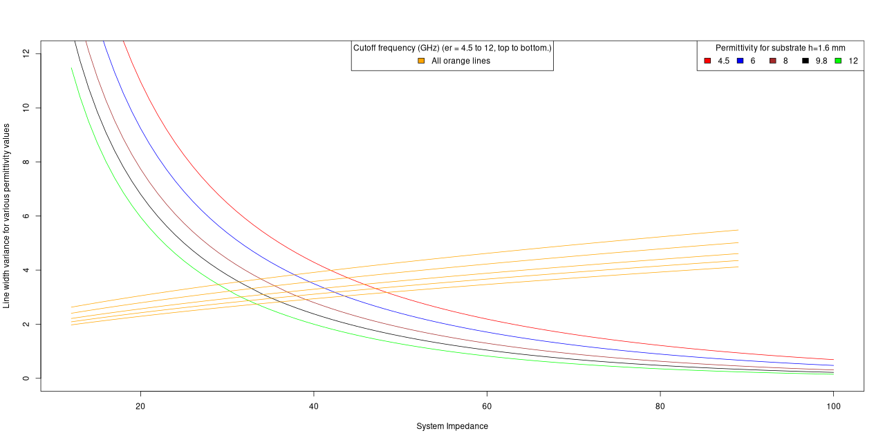
This first chart shows the changes for substrate = 1.6 mm. Next is showing widths on a 0.813 mm board. Easily seen is the thinner board allows thinner lines for the same impedance values.
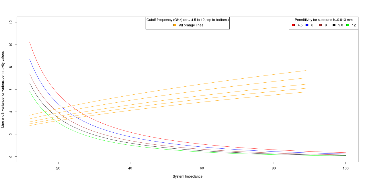
Also note the width variances decrease as the impedance becomes higher, regardless of board thickness. Comparing the two charts readily shows that the cutoff frequency, fo, below which dispersion can be ignored, is lower for thicker substrates. However, the cutoff frequency is slightly higher for lower er values, which is rather non-intuitive.
Praise God for giving me the insights to discover ways to generate these charts using (Allaire et al. 2023) and (R Core Team 2023). I attempted to use (Wickham et al. 2023) to generate the charts, but it only accepts the data.frame format as input, whereas I placed my data in an array format, because the array has multiple dimensions (x,y,z (or slices)). When I converted it into a data frame, the data was scrambled. So rather than redesign the data storage format, I just used the standard plot() function. Then, by adding lines() to the basic plot, I created the charts you see here.
References
Footnotes
W.J. Getsinger, “Microstrip Dispersion,” Proc. IEEE, Vol. 60, pp. 144-146, (January, 1972).↩︎