Casual Microstrip Design 2
In the first post of the same title, we explored preliminary methods for designing a microstrip line using references (Edwards and Steer 2016) and (Pozar 2012). In this second post, we will continue, with some overlap, the process to determine a filter.
Now we enter into the whole purpose for these efforts, determining the impedance values for a bandpass filter. We will use an example found elsewhere so we have a cross-reference for the results. This is a design for a GPS bandpass filter1. The values used are for a third-order Chebyshev filter design for a frequency of 1575 MHz using a Rogers 4003 board, whereas we are using FR4 board. So, the end results are somewhat different.
- Board:
- er = 4.5.
- substrate = 1.57.
- copper = 35 um.
- Center frequency = 1575 MHz.
- Lower frequency = 1550 MHz.
- Upper frequency = 1600 MHz.
- Ripple factor = 0.01.
- Filter order = 3.
- System impedance (ZO) = 50 ohms.
At this higher frequency, losses and ripple are difficult to control for FR4 board. A better board would be Rogers 4003. At any rate, the first factors we need to determine are the normalized values for the components. Using R, these are the formulae:
\[beta = log\left(\frac{\cosh(ripple/17.37)}{\sinh(ripple/17.37}\right)\] \[y = \sinh\left(\frac{beta}{2 * order}\right)\]
There must be one more pair than the desired filter order (i.e., N of 3 = 4 pairs). Two additional calculations are required for each pair. An easy way to store those values in R is a matrix or data.frame.
The additional formulae using count=1 to N are:
\[x_{count} = \sin\left(\frac{2*count * \pi}{2N}\right) \hspace{8pt} and \hspace{8pt} z_{count} = y^2 + \sin\left(\frac{count * \pi}{N}\right)^2\]
After looping through each count and saving the values, we then determine the first normalized value as so: \(G_1 = 2 * x_1 / y\). For the remaining G values:
\[G_{count} = \frac{4 * x_{count-1} * x_{count}}{z_{count-1} * G_{count-1}}\]
In the above referenced article, another program (faisyn) was used to determine the normalized values, which broke the calculation chain. That’s why I have recreated the formulae here. The Rload value for odd-N orders will be 1. The normalized values are:
- g1 = 0.6291
- g2 = 0.9702
- g3 = 0.6291
- Rload 1
Next step was to determine the fractional bandwidth simply as:
\[\triangle = \frac{ f_{max} - f_{min}}{f_{mean}} = 0.031746\]
This value is used in the admittance inverter constant calculations for each pair.
\[Z_o.J_1 = \sqrt{\frac{\pi * \triangle}{2 * g_1}} = 0.28154\] \[Z_o.J_2 = \frac{\pi * \triangle}{2 * \sqrt{g_1 * g_2}} = 0.06383\] \[Z_o.J_3 = \frac{\pi * \triangle}{2 * \sqrt{g_2 * g_3}} = 0.06383\] \[Z_o.J_1 = \sqrt{\frac{\pi * \triangle}{2 * g_3 * g_4}} = 0.28154\]
Each line pair even/odd impedances are calculated as such:
\[Z_{EVEN} = Z_O * \lvert 1 + Z_o.J_N + (Z_o.J_N)^2 \rvert\] \[Z_{ODD} = Z_O * \lvert 1 - Z_o.J_N + (Z_o.J_N)^2 \rvert\]
That gives us the even/odd impedances in ohms (@ 90o) for our microstrip line pairs.
- Even Odd
- 68.04 39.89
- 53.40 47.01
- 53.40 47.01
- 68.04 39.89
We now have what we need to create an actual filter design using (Wedge, Compton, and Rutledge 1991).
PUFF CAD program.
If we enter these values into PUFF as ‘clines’, we can determine the performance of the filter. We set up PUFF [BOARD] factors from the list above, then create two ‘cline’ entries in the [PARTS] box, formatted as: \(\hspace{8pt} cl! \hspace{8pt} 68.04\Omega \hspace{8pt} 39.89\Omega \hspace{8pt} 90^o\) and \(\hspace{8pt} cl! \hspace{8pt} 53.40\Omega \hspace{8pt} 47.01\Omega \hspace{8pt} 90^o\). The area for entries in the [PARTS] is tight, so the above spaces are not necessary, but are shown for clarity. In PUFF, the symbols for ohms (\(\Omega\)) and degrees (o) are entered with CTRL-O and CTRL-D. The ‘!’ in the ‘cline’ allows PUFF to compensate for dispersion losses and other factors, and will modify the actual values. So it is necessary to adjust the values by pressing ‘=’ while in the [PARTS] box on the desired part. The actual values are shown directly above in a red box. Change the ‘cline’ values to bring those values back to the calculated values.
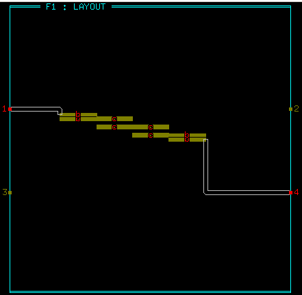
Figure 1 shows the ‘cline’ layout, where the first ‘cline’ is at each end, and the second ‘cline’ is in the center twice. Connection to port 4 is only to make the connections look clearer. Normal values would be S11 and S21, but S41 looks neater, and doesn’t affect the actual parameters. The return reflection shows -1.31 dB loss at 0.1o phase angle. These values are after adjustment. To see the physical dimensions, remove the ‘!’ from the ‘cline’ to read the width and length, again by pressing ‘=’.
For a real circuit, fringing effect end corrections must be applied, which will shorten the lines a bit. For coupled lines, the value would be negative, but only half of the calculated length. Determine the length extension (l) using:
\[\frac{l}{h} = 0.412 \left(\frac{e_{re} + 0.3}{e_{re} - 0.258}\right) \left(\frac{w/h _ 0.262}{w/h + 0.813}\right)\]
where ‘h’ is substrate thickness. The value, ’ere, referenced in (Hammerstad and Bekkadal 1975) (which is out of print), is vague, but there is a chart (See Table 7.2 below) in Chapter 7 of the PUFF manual which allows determining length correction ratio, given Zo and er values, and is much easier than the above formula. Then the extension, \(\ell_{eo} = \frac{ratio \times dielectric}{2}\) for the half value.
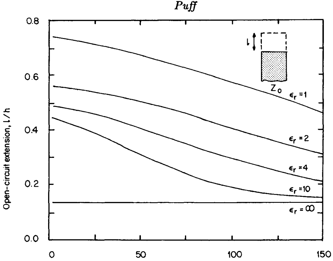
Further study shows the above empirical formula is also depicted in Chapter 9 of (Edwards and Steer 2016), but where ’ere is replaced with Eeff. It also indicates errors can exceed 5%, which can be significant for filter design.
\[\ell_{eo} = 0.412 h \left(\frac{E_{eff} + 0.3}{E_{eff} - 0.258}\right) \left(\frac{w/h + 0.262}{w/h + 0.813}\right)\]
where Eeff is defined here. So, using a board of er=9.8, h=0.813 mm, a 90o line at 1575 MHz and Zo=50 ohms gives a ratio of 0.310 which coincides with the above chart. This gives an extension of 0.126 to be subtracted from the open end of a coupled microstrip.
It is worthwhile to acquire a copy of the PUFF manual, if only for the information. PUFF is released in the public domain under the GPL license, and can be acquired for both PC and Linux operating systems. The manual copy usually comes with the package2.
And, I did manage to develop a ‘R’ file to calculate all the parameters for entry to PUFF. Saves a lot of work and potential mistakes when working the formulae.
We thank God for the insights we may not have thought of ourselves. Have a great day.