Casual Microstrip Design
Some years ago (~20), I was dabbling in the mysterious world of microwave design (and I still do to a lesser extent), and was looking at various formulas to determine dimensions for microstrip widths and lengths. I had two paths to investigate, namely, recent references by (Edwards and Steer 2016) and (Pozar 2012). That’s because those were the two reference books I had. Terry Edward’s book seems more in-depth with a nuts-and-bolts approach, where David Pozar’s volume is more a macro-level dissertation of the subject. Both books are chock full of useful information for microwave design, and generally follow the same paths, and although the results are similar, there are slight differences in final dimensions.
1: Edwards: Foundations for Microstrip Circuit Design.
Firstly, I will depict the formulas I have used for years for determining dimensions. I generally neglect dispersion, fringing effects, etc., especially at lower frequencies. Chapter 7 of (Edwards and Steer 2016) covers dispersion at higher frequencies. For in-depth analysis, there is no replacement for actually studying the book.
The formulas I show here, from Edward’s book, are closed formulas for static-TEM1 designs. There are two types of microstrips, high impedance and low impedance, and the formulas are different. Narrow strips are defined where desired impedance, \(Z_o > (44 - 2e_r) \Omega\). Wide strips are where impedance, \(Z_o < (44 - 2e_r) \Omega\).
High impedance, narrow strips.
For determining the ratio of microstrip width (w) to substrate thickness (h), we use the formulas below. As H’ is used in the w/h formula, we determine it first:
\[H' = \frac{Z_o \sqrt{2(e_r + 1)}}{119.9} + \frac{1}{2} \left(\frac{e_r - 1}{e_r + 1}\right) \left(ln\frac{\pi}{2} + \frac{1}{e_r} ln\frac{4}{\pi}\right)\]
and then:
\[\frac{w}{h} = \left(\frac{e^{H'}}{8} - \frac{1}{4 e^{H'}}\right)^{-1}\]
where Euler’s number, e = 2.718281828, and \(e_r\) is relative permittivity2 of the board substrate. Now, to determine the effective relative permittivity:
\[ E_{eff} = \frac{e_r + 1}{2} \left[1 - \frac{1}{2H'} \left(\frac{e_r - 1}{e_r + 1}\right) \left(ln \frac{\pi}{2} + \frac{1}{e_r} ln \frac{4}{\pi} \right) \right]^{-2}\]
Low impedance, wide strips.
For wide strips, the formula is a bit different. As above we first determine one of the variables \(d_e\). The w/h formula from Edwards has two variables, der and de1. However, the difference in output is barely noticeable, so I will make a little jump here and use \(d_e = \frac{59.95\pi^2}{Z_o \sqrt{e_r}}\) for both in the below w/h formula. I decided this by cross-referencing the (Wedge, Compton, and Rutledge 1991) book for CAD microwave design, the ubiquitous PUFF.
\[\frac{w}{h} = \frac{2}{\pi} [(d_e - 1) - ln(2 d_e - 1)] + \frac{(e_r - 1)}{\pi e_r} \left[ ln(d_e -1) + 0.293 - \frac{0.517}{e_r} \right]\]
Final dimensions.
Determining the microstrip width is simply substrate thickness (h) divided by inverse w/h ratio, \(w = \frac{h}{w/h^{-1}}\). As I wanted to make it easier to program this on my handheld calculator, I broke up the following formula as so:
\[A = 1.0 + \left[ln\left(e^{4 ln\frac{w}{h}} + \left(\frac{w}{h}/52\right)^2\right) / \left(e^{4 ln\left(\frac{w}{h}\right)} +0.432/49\right)\right] \] \[+ \left[ln\left((1+e^{3ln\frac{w/h}{18.1}}\right) / 18.7 \right] \]
\[ B = 0.564 e^{0.053 ln \frac{e_r - 0.9}{e_r + 3.0}} \]
\[ C = \frac{e_r + 1.0}{2} + \left[\frac{e_r - 1.0}{2} \times e^{-A B ln\left(1.0 + \frac{10}{w/h}\right)}\right] \]
Finally, the microstrip length (\(\ell\)) is deduced by the desired phase angle (\(\phi\)) such:
\[ \ell = (\phi \times \frac{c}{freq / \sqrt{C}} / 360) \times 1000 \] where lightspeed (c) = 2.99792458e8.
So now, let’s use an example to show the process and determine some useful results. We could use an alumina substrate with thickness (h) 0.6mm, relative permittivity (er) 9.8 and dielectric loss tan (\(\delta\)) 0.001, at a frequency of 2 GHz with a phase angle (\(\phi\)) of 90o and input impedance (Zo) of 50 \(\Omega\).
Those parameters give us the following results:
- w/h = 0.976
- Eeff = 6.555
- width = 0.586 mm
- length = 14.636 mm
At higher frequencies, dispersion calculations would be required, detailed in Chapter 7 of (Edwards and Steer 2016).
2: Pozar: Microwave Engineering
So, from Pozar’s formulas, where the w/h ratio is less than 2, we use the following:
\[\frac{w}{h} = \frac{8 e^A}{e^{2 A} - 2}\]
where
\[A = \frac{Z_o}{60} \sqrt{\frac{e_r + 1}{2}} + \frac{e_r - 1}{e_r + 1} \left(0.23 + \frac{0.11}{e_r}\right)\]
If the w/h ratio is greater than 2, we use this formula:
\[\frac{w}{h} = \frac{2}{\pi} \left[ B - 1 - ln(2 B - 1) + \frac{e_r - 1}{2 e_r} \left( ln(B - 1) + 0.39 - \frac{0.61}{e_r} \right) \right]\]
where
\[B = \frac{377 \pi}{2 Z_o \sqrt{e_r}}\]
Final dimensions.
We once again determine the width as such:
\[w = \frac{h}{w/h^{-1}}\]
And, for a slightly different way to determine length, we first find the effective dielectric constant (ee) of the microstrip line with:
\[e_e = \frac{e_r +1}{2} + \frac{e_r - 1}{2} \times \frac{1}{\sqrt{1 + 12 h / w}}\]
and with \(k_o = \frac{2 \pi f}{c}\), we find the length:
\[ \ell = \frac{\phi (\pi / 180^o)}{\sqrt{e_e} k_o}\]
For a higher frequency example, we again use an alumina substrate with thickness (h) 0.6mm, relative permittivity (er) 9.8 and dielectric loss tan (\(\delta\)) 0.001, at a frequency of 10 GHz with a phase angle (\(\phi\)) of 270o and input impedance (Zo) of 50 \(\Omega\). This gives the following results:
- w/h = 0.975
- Eeff = 6.508
- width = 0.4876 mm
- length = 8.8136 mm
3: PUFF Microwave Examination.
We now plug these values into the PUFF CAD program, which I still like as an investigative tool. I first used this back in the ’90s on Windows/DOS. Now I am using it on Linux, and it still works just as well. Using the first example, Puff shows a width of 0.587 mm, and a length of 14.473 mm. The second example shows width 0.587 mm with length 8.684 mm. These values are not as close as they should be, but that is with no effort made for optimization.
Summary.
This has been a casual treatise exploring different methods from two different reference volumes, and is in no way rigorous, from a scientific viewpoint. It is a way to reacquaint myself with some microwave formulas. I am attempting to recreate this in “R” from my Casio Prizm just for the fun of it.
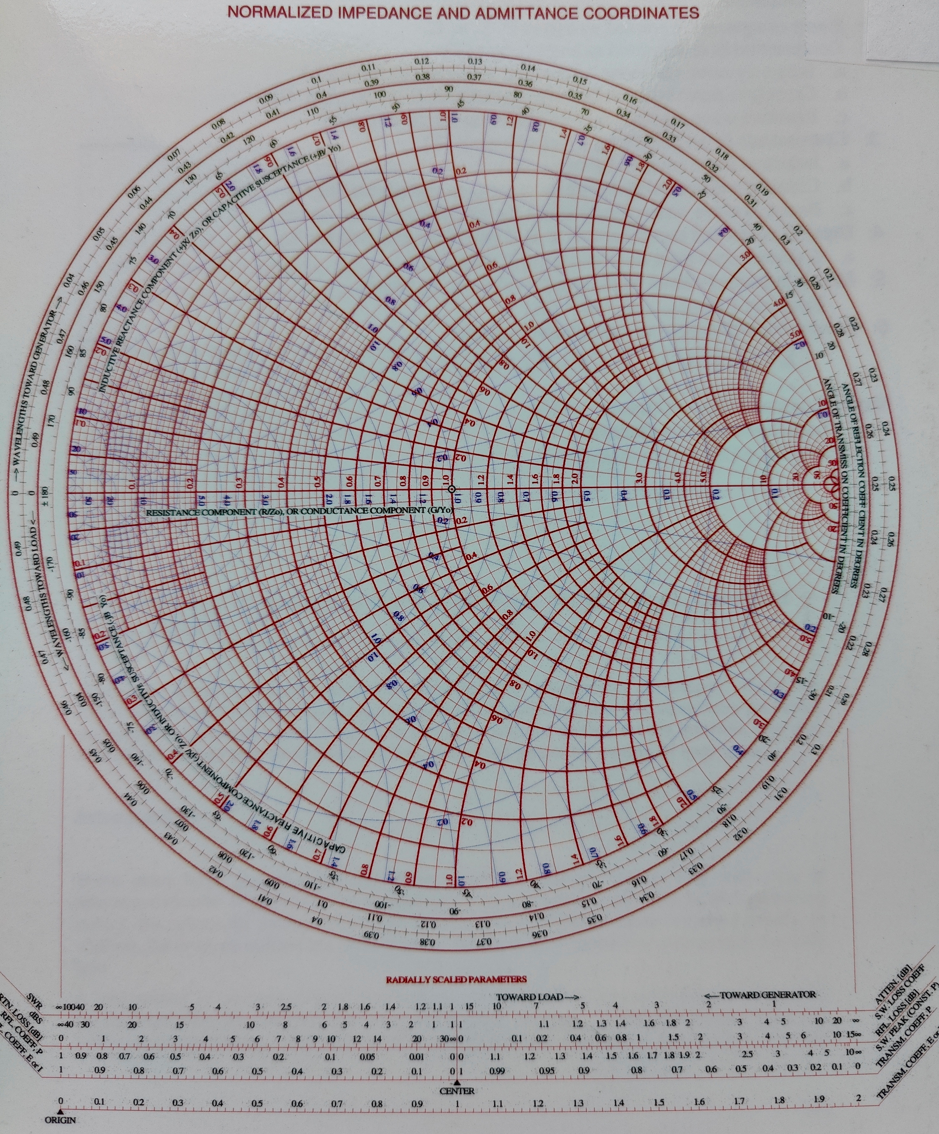
So that’s it for this post. Again we thank God for everything we have and are. BTW, here is a full resolution image of the Smith Chart shown in the header. Have a great day! See Ya Next Year!